Before we start the topic lets understand the few fundamental concepts

Fine-tuning vs Pre-training

Pre-training involves training a model on a large dataset to learn general features and patterns.

Fine-tuning is the process of taking a pretrained machine learning model and further training it on a smaller, targeted data set. The aim of fine-tuning is to maintain the original capabilities of a pretrained model while adapting it to suit more specialized use cases.

Instruction fine tuning / Full fine tuning

Catastrophic Forgetting

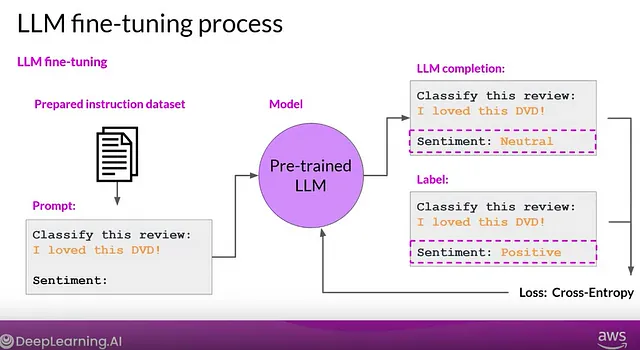
Fine tuning can significantly increase the performance of a model on a specific task but can lead to reduction in ability on other tasks.

Multitask fine tuning

It can help to reduce the impact of catastrophic forgetting but many example of each task will be needed.

Parameter efficient fine-tuning (PEFT)

PEFT approaches helps to get performance comparable to full fine-tuning while only having a small number of trainable parameters. This also overcomes the issues of catastrophic forgetting, a behavior observed during the full fine-tuning of LLMs. PEFT approaches have also shown to be better than fine-tuning in the low-data regimes and generalize better to out-of-domain scenarios.

1. Low-rank Adaptation, or LoRA

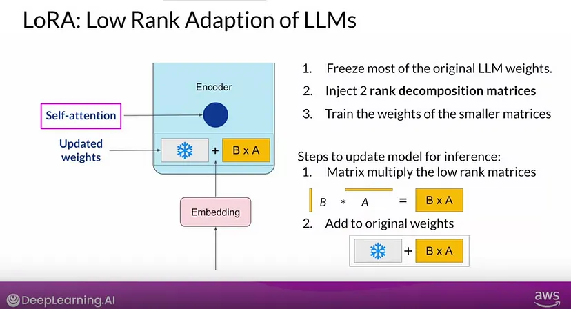
Training a LLM to update all the model weight can be very expensive due to GPU memory limitations. Among the PEFT methods LORA is the most efficient technique for training custom LLM which needs few parameters for training.

For simplicity lets consider a LLM which contains only 1 weight matrix W. While training the model the optimizer will calculate the gradient estimate ΔW based on the loss function (in other words the backpropagation process). Then weight update is

Wupdated = W + ΔW

If the weight matrix W contains 7B parameters, then the weight update matrix ΔW also contains 7B parameters, and computing the matrix ΔW can be very compute and memory intensive.

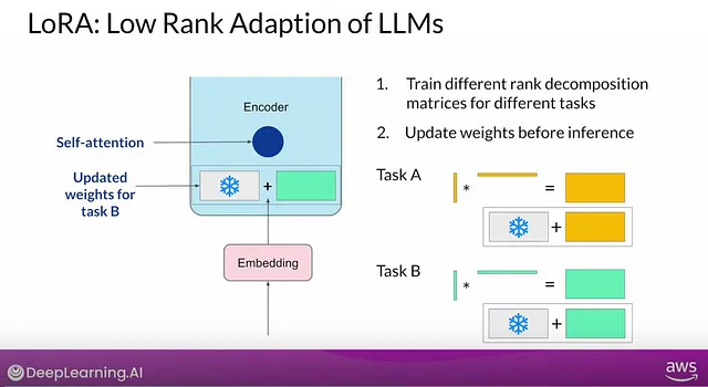
The LoRA method replaces the ΔW into a lower-rank representation. LoRA learns the decomposed representation of ΔW directly during training which is where the savings are coming from, as shown in the figure below.

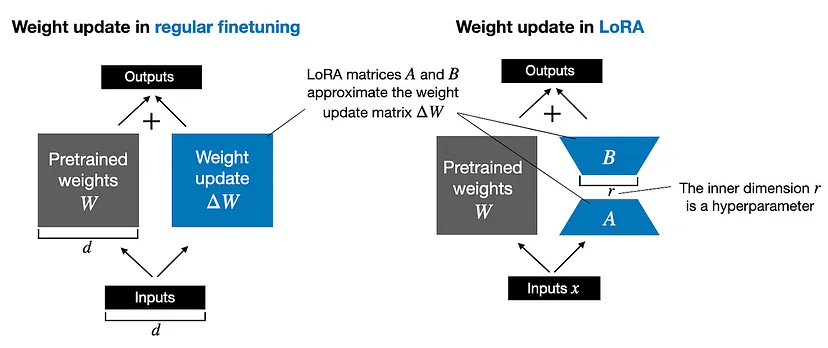
As illustrated above, the decomposition of ΔW in to two smaller LoRA matrices, A and B. If A has the same number of rows as ΔW and B has the same number of columns as ΔW, we can write the decomposition as ΔW = AB. (AB is the matrix multiplication result between matrices A and B.) The rank r is the hyperparameter which decides how much memory will be saved.

How to choose the rank of the LoRA matrices?
The selection of the rank for LoRA matrices is an ongoing research topic. Lower ranks reduce the number of trainable parameters, saving on computation. However, model performance must be considered. A rank between 4 and 32 is suggested as a good balance between reducing parameters and maintaining performance. Choosing an r that is too large could result in more overfitting. On the other hand, a small r may not be able to capture diverse tasks in a dataset.

2. Prompt Tuning

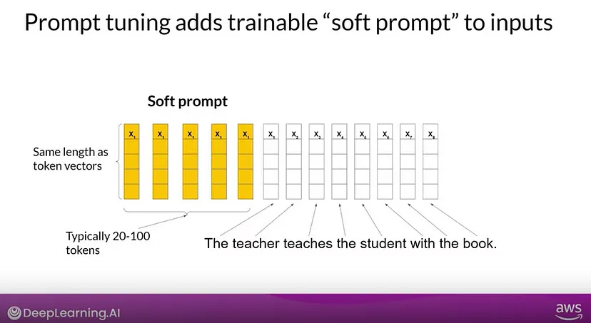
In prompt tuning, additional trainable tokens, known as a soft prompt, are added to the prompt. The supervised learning process determines their optimal values. These soft prompt vectors, which have the same length as the language token embedding vectors, are prepended to your input text’s embedding vectors. Including between 20 and 100 virtual tokens can yield good performance.

In full fine tuning, the training data set consists of input prompts and output completions or labels, and the weights of the large language model are updated during supervised learning. Unlike prompt tuning, the weights of the large language model are frozen in full fine tuning. Instead, the soft prompt’s embedding vectors are updated over time to optimize the model’s completion of the prompt.

3. Adapters

This method involves adding extra layers to the existing transformer model and fine-tuning only these layers, which has been shown to yield comparable results to full model fine-tuning. The modified transformer architecture includes adapter layers added after the attention and feed-forward stacks. These adapter layers employ a bottleneck design, reducing the input to a smaller dimension, applying a non-linear activation function, and then expanding it back to the input dimension, ensuring compatibility with the subsequent transformer layer.

During training this approach is compute efficient, but problem is the large models are parallelized on hardware while adapter layers must be processed in sequentially. this means that during inference the adapters introduce a noticeable latency.